Py: Image Recognition

This notebook was originally created by Elliot Dawson for the Data Analytics Applications subject, as Case Study 2 in DAA M05 Classification and neural networks

Data Analytics Applications is a Fellowship Applications (Module 3) subject with the Actuaries Institute that aims to teach students how to apply a range of data analytics skills, such as neural networks, natural language processing, unsupervised learning and optimisation techniques, together with their professional judgement, to solve a variety of complex and challenging business problems. The business problems used as examples in this subject are drawn from a wide range of industries.

Find out more about the course here.

Define the Problem:

Another popular use of neural networks is in image detection. Examples of ways in which neural network image classifiers might be used to solve business problems include:

• analysing drone images to make the insurance claims management process more efficient, such as by classifying the level of damage caused to a property following a natural disaster; and

• extracting information from handwritten correspondence from customers, such as information on insurance claims forms to be entered into the claims database.

This case study investigates the use of a neural network to decipher handwritten digits (from zero to nine). This might be a useful tool if, for example, you are trying to automate the process of sorting mail based on postcodes written on the front of envelopes. Of course, the task of training a neural network to recognise hand-written digits can also be extended to recognising hand-written letters and then words.

Purpose:

This case study by Elliot Dawson involves building neural networks to recognise handwritten digits from zero to nine. The case study also compares the performance of the neural networks built to the performance of a gradient boosting machine (GBM) built to solve the same problem.

References:

The dataset used in this case study is a famous Modified National Institute of Standards and Technology (MNIST) dataset of handwritten images (http://yann.lecun.com/exdb/mnist/). The MNIST dataset is popular for use in benchmarking classification algorithms.

The dataset has 42,000 observations, each representing a greyscale image of a hand-drawn digit from zero to nine. Each image is 28 pixels in height and 28 pixels in width, making a total of 784 pixels (28x28). Each pixel has a single pixel value associated with it, from 0 to 255, indicating the lightness or darkness of that pixel. Higher pixel values represent darker pixels. The dataset represents these images as 784 features, with each feature representing a different pixel in the image.

The dataset also contains one response (‘label’) that takes integer values from zero to nine, indicatating the digit drawn in each image.

Packages

This section imports the packages that will be required for this exercise/case study.

We’ll use:

• pandas for data management

• numpy for mathematical operations

• Support functions from matplotlib, sklearns, seaborn packages

• keras, from the tensorflow package, for fitting the neural networks

import pandas as pd # For data management.
import numpy as np # For mathematical operations.

# Matplotlib and Seaborn are used for plotting.
import matplotlib.pyplot as plt
import matplotlib.image as mpimg
import seaborn as sns
%matplotlib inline

# Various scikit-learn functions to help with modelling and diagnostics.
from sklearn.model_selection import train_test_split
from sklearn.metrics import confusion_matrix
import itertools

# Keras, from the Tensorflow package, is used for fitting the neural networks.
from keras.utils.np_utils import to_categorical
from keras.models import Sequential
from keras.layers import Dense, Dropout, Flatten, Conv2D, MaxPool2D
from keras.optimizers import RMSprop, SGD
from keras.preprocessing.image import ImageDataGenerator
from keras.callbacks import ReduceLROnPlateau
from tensorflow.keras.utils import plot_model

import os

Functions

This section defines functions that will be used for this exercise/case study.

# Define a function to split the data into train, validation, and test sets.
# This function uses the train_test_split function from the sklearn package
# to do the actual data splitting.

def create_data_splits(dataset, response_col):
    # Split data into train/test (80%, 20%).
    train_full, test = train_test_split(dataset, test_size = 0.2, random_state = 123)

    # Create a validation set from the training data (20%).
    train, validation = train_test_split(train_full, test_size = 0.2, random_state = 234)

    # Create train and validation model matrices and response vectors.
    # For the response vector, convert Churn Yes/No to 1/0

    train_x = train.drop(labels=response_col, axis=1)
    train_y = train[response_col]
    train_y.index = range(len(train_y))

    validation_x = validation.drop(labels=response_col, axis=1)
    validation_y = validation[response_col]
    validation_y.index = range(len(validation_y))

    test_x = test.drop(labels=response_col, axis=1)
    test_y = test[response_col]
    test_y.index = range(len(test_y))

    return train_x, train_y, validation_x, validation_y, test_x, test_y

# Define a function to generate a confusion matrix to observe a model's results.
def plot_confusion_matrix(cm, classes,
                          normalise=False,
                          title='Confusion matrix',
                          cmap=plt.cm.Blues):
    '''
    This function prints and plots a confusion matrix.
    Normalisation of the matrix can be applied by setting `normalise=True`.
    Normalisation ensures that the sum of each row in the confusion matrix is 1.
    '''
    plt.imshow(cm, interpolation='nearest', cmap=cmap)
    plt.title(title)
    plt.colorbar()
    tick_marks = np.arange(len(classes))
    plt.xticks(tick_marks, classes, rotation=45)
    plt.yticks(tick_marks, classes)

    if normalise:
        cm = cm.astype('float') / cm.sum(axis=1)[:, np.newaxis]

    thresh = cm.max() / 2.
    for i, j in itertools.product(range(cm.shape[0]), range(cm.shape[1])):
        plt.text(j, i, cm[i, j],
                 horizontalalignment='center',
                 color='white' if cm[i, j] > thresh else 'black')

    plt.tight_layout()
    plt.ylabel('True response')
    plt.xlabel('Predicted response')

Data

This section:

• imports the data that will be used in the modelling;

• explores the data; and

• prepares the data for modelling.

Import data

The code below reads the CSV into a pandas data frame.

Note that the MNIST dataset is large (75MB) hence it has been zipped, but pandas reads it natively.

# Specify the folder or URL datasets are saved in.
infolder = 'https://actuariesinstitute.github.io/cookbook/_static/daa_datasets/'

# Specify the filename.
file = 'DAA_M05_CS2_data.csv.zip'

# Read in the data from your Google Drive folder.
dataset = pd.read_csv (infolder+file)

Explore data (EDA)

Prior to commencing any modelling, the code below observes:

• the features in the dataset and their types;

• the count of the number of observations for each response class.

Graphical observations of the images will be made later in the notebook once the data has been pre-processed.

# Check the types of each feature and the response variable ('label').
dataset.dtypes

label       int64
pixel0      int64
pixel1      int64
pixel2      int64
pixel3      int64
            ...  
pixel779    int64
pixel780    int64
pixel781    int64
pixel782    int64
pixel783    int64
Length: 785, dtype: object

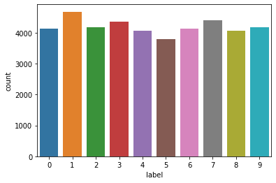
# Extract the counts for each response class (digit) and build a barplot of these
# counts for each of interpretation.
sns.countplot(x='label',data=dataset)
print(dataset['label'].value_counts())

1    4684
7    4401
3    4351
9    4188
2    4177
6    4137
0    4132
4    4072
8    4063
5    3795
Name: label, dtype: int64

Prepare data

The dataset will be pre-processed so that neural networks can be built with the data.

## Split the dataset into a train, validation, and test set. 
train_x, train_y, validation_x, validation_y, test_x, test_y \
= create_data_splits(dataset, 'label')

# Rescale the features from being in the range [0,255] to [0:1].
train_x = train_x/255.0
validation_x = validation_x/255.0
test_x = test_x/255.0

# Reshape the features for each observation from being a vector of size 784
# to being a matrix of size 28x28.
# This is required for building the convolutional neural network (CNN) below.
train_cnn_x = train_x.values.reshape(-1, 28, 28, 1)
validation_cnn_x = validation_x.values.reshape(-1, 28, 28, 1)
test_cnn_x = test_x.values.reshape(-1, 28, 28, 1)

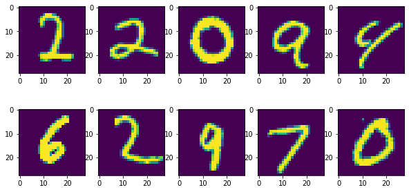
View observations

The code below visualises an observation (hand-written digit) from each of the response classes.

# Visualise an example from each of the response classes
# (the digits from 0 to 9).
fig = plt.figure(figsize=(10,5))
rows = 2
columns = 5
for i in range(0, 10):
    fig.add_subplot(rows, columns, i+1)
    plt.imshow(train_cnn_x[train_y[train_y == i].index[0]][:,:,0])
plt.show()

# Encode the response from a continuous (integer) to a categorical variable.
train_y = to_categorical(train_y, num_classes=10)
validation_y = to_categorical(validation_y, num_classes=10)
test_y = to_categorical(test_y, num_classes=10)

Modelling

This section:

• fits a model;

• evaluates the fitted model;

• improves the model; and

• selects a final model.

Fit a ‘vanilla’ neural network (NN 1)

The code below uses Keras to construct a neural network with:

• two hidden layers, each with 16 neurons and the ReLU activation function; and

• one output layer with 10 neurons (representing each of the digits from zero to nine) and the softmax activation function.

# Specify the model's architecture.
nn_model = Sequential()
nn_model.add(Dense(16, input_dim= 784, kernel_initializer='normal', activation='relu'))
nn_model.add(Dense(16, activation='relu', kernel_regularizer='l2'))
nn_model.add(Dense(10, activation='softmax'))

# Compile the model.
opt = SGD(learning_rate=0.2, momentum=0.0)
  # This specifies that regular stochastic gradient descent (SGD) should be
  # used with a learning rate of 0.2.
  # Momentum = 0 specifies that the regular SGD algorithm should be used
  # 'without momentum'.
  # SGD with momentum is a variant on regular SGD that uses an
  # exponential moving average of current and past gradients rather than just
  # the gradient for the current iteration.
nn_model.compile(
    loss='categorical_crossentropy', 
      # The 'categorical_crossentropy' loss function is useful
      # for an integer response variable.
    optimizer =  opt,

    metrics=['accuracy'],
)
nn_hist = nn_model.fit(np.array(train_x), np.array(train_y), epochs=100,batch_size=1000, validation_data = (validation_x, validation_y))

Epoch 1/100
27/27 [==============================] - 10s 21ms/step - loss: 2.2099 - accuracy: 0.2815 - val_loss: 1.5056 - val_accuracy: 0.5580
Epoch 2/100
27/27 [==============================] - 0s 4ms/step - loss: 1.2441 - accuracy: 0.6751 - val_loss: 1.0109 - val_accuracy: 0.7324
Epoch 3/100
27/27 [==============================] - 0s 4ms/step - loss: 0.8064 - accuracy: 0.8128 - val_loss: 0.6254 - val_accuracy: 0.8704
Epoch 4/100
27/27 [==============================] - 0s 6ms/step - loss: 0.6322 - accuracy: 0.8601 - val_loss: 0.5649 - val_accuracy: 0.8813
Epoch 5/100
27/27 [==============================] - 0s 4ms/step - loss: 0.5453 - accuracy: 0.8848 - val_loss: 0.5192 - val_accuracy: 0.8894
Epoch 6/100
27/27 [==============================] - 0s 5ms/step - loss: 0.5109 - accuracy: 0.8878 - val_loss: 0.4891 - val_accuracy: 0.8958
Epoch 7/100
27/27 [==============================] - 0s 4ms/step - loss: 0.4799 - accuracy: 0.8963 - val_loss: 0.4731 - val_accuracy: 0.8969
Epoch 8/100
27/27 [==============================] - 0s 5ms/step - loss: 0.4613 - accuracy: 0.8972 - val_loss: 0.4463 - val_accuracy: 0.9006
Epoch 9/100
27/27 [==============================] - 0s 4ms/step - loss: 0.4240 - accuracy: 0.9088 - val_loss: 0.4260 - val_accuracy: 0.9037
Epoch 10/100
27/27 [==============================] - 0s 4ms/step - loss: 0.4239 - accuracy: 0.9051 - val_loss: 0.4166 - val_accuracy: 0.9055
Epoch 11/100
27/27 [==============================] - 0s 4ms/step - loss: 0.4069 - accuracy: 0.9097 - val_loss: 0.3972 - val_accuracy: 0.9094
Epoch 12/100
27/27 [==============================] - 0s 4ms/step - loss: 0.4006 - accuracy: 0.9084 - val_loss: 0.3894 - val_accuracy: 0.9101
Epoch 13/100
27/27 [==============================] - 0s 4ms/step - loss: 0.3797 - accuracy: 0.9142 - val_loss: 0.3957 - val_accuracy: 0.9082
Epoch 14/100
27/27 [==============================] - 0s 5ms/step - loss: 0.3699 - accuracy: 0.9154 - val_loss: 0.3702 - val_accuracy: 0.9146
Epoch 15/100
27/27 [==============================] - 0s 5ms/step - loss: 0.3464 - accuracy: 0.9215 - val_loss: 0.3825 - val_accuracy: 0.9097
Epoch 16/100
27/27 [==============================] - 0s 4ms/step - loss: 0.3588 - accuracy: 0.9170 - val_loss: 0.3644 - val_accuracy: 0.9146
Epoch 17/100
27/27 [==============================] - 0s 4ms/step - loss: 0.3460 - accuracy: 0.9204 - val_loss: 0.3608 - val_accuracy: 0.9159
Epoch 18/100
27/27 [==============================] - 0s 4ms/step - loss: 0.3409 - accuracy: 0.9215 - val_loss: 0.3529 - val_accuracy: 0.9186
Epoch 19/100
27/27 [==============================] - 0s 5ms/step - loss: 0.3302 - accuracy: 0.9220 - val_loss: 0.3485 - val_accuracy: 0.9170
Epoch 20/100
27/27 [==============================] - 0s 4ms/step - loss: 0.3380 - accuracy: 0.9185 - val_loss: 0.3405 - val_accuracy: 0.9192
Epoch 21/100
27/27 [==============================] - 0s 4ms/step - loss: 0.3135 - accuracy: 0.9294 - val_loss: 0.3444 - val_accuracy: 0.9189
Epoch 22/100
27/27 [==============================] - 0s 4ms/step - loss: 0.3127 - accuracy: 0.9286 - val_loss: 0.3367 - val_accuracy: 0.9193
Epoch 23/100
27/27 [==============================] - 0s 4ms/step - loss: 0.3137 - accuracy: 0.9281 - val_loss: 0.3713 - val_accuracy: 0.9040
Epoch 24/100
27/27 [==============================] - 0s 4ms/step - loss: 0.3454 - accuracy: 0.9149 - val_loss: 0.3292 - val_accuracy: 0.9207
Epoch 25/100
27/27 [==============================] - 0s 4ms/step - loss: 0.3047 - accuracy: 0.9282 - val_loss: 0.3552 - val_accuracy: 0.9113
Epoch 26/100
27/27 [==============================] - 0s 7ms/step - loss: 0.3171 - accuracy: 0.9241 - val_loss: 0.4023 - val_accuracy: 0.8930
Epoch 27/100
27/27 [==============================] - 0s 5ms/step - loss: 0.3202 - accuracy: 0.9231 - val_loss: 0.3204 - val_accuracy: 0.9231
Epoch 28/100
27/27 [==============================] - 0s 4ms/step - loss: 0.2993 - accuracy: 0.9312 - val_loss: 0.3280 - val_accuracy: 0.9189
Epoch 29/100
27/27 [==============================] - 0s 5ms/step - loss: 0.2936 - accuracy: 0.9330 - val_loss: 0.3078 - val_accuracy: 0.9269
Epoch 30/100
27/27 [==============================] - 0s 4ms/step - loss: 0.2880 - accuracy: 0.9308 - val_loss: 0.3068 - val_accuracy: 0.9265
Epoch 31/100
27/27 [==============================] - 0s 4ms/step - loss: 0.2944 - accuracy: 0.9294 - val_loss: 0.3418 - val_accuracy: 0.9112
Epoch 32/100
27/27 [==============================] - 0s 4ms/step - loss: 0.2891 - accuracy: 0.9311 - val_loss: 0.3098 - val_accuracy: 0.9254
Epoch 33/100
27/27 [==============================] - 0s 4ms/step - loss: 0.2817 - accuracy: 0.9327 - val_loss: 0.3269 - val_accuracy: 0.9165
Epoch 34/100
27/27 [==============================] - 0s 5ms/step - loss: 0.2825 - accuracy: 0.9340 - val_loss: 0.3027 - val_accuracy: 0.9265
Epoch 35/100
27/27 [==============================] - 0s 4ms/step - loss: 0.2914 - accuracy: 0.9286 - val_loss: 0.3074 - val_accuracy: 0.9250
Epoch 36/100
27/27 [==============================] - 0s 5ms/step - loss: 0.2730 - accuracy: 0.9333 - val_loss: 0.2950 - val_accuracy: 0.9292
Epoch 37/100
27/27 [==============================] - 0s 4ms/step - loss: 0.2721 - accuracy: 0.9356 - val_loss: 0.3119 - val_accuracy: 0.9214
Epoch 38/100
27/27 [==============================] - 0s 4ms/step - loss: 0.2742 - accuracy: 0.9357 - val_loss: 0.3431 - val_accuracy: 0.9110
Epoch 39/100
27/27 [==============================] - 0s 5ms/step - loss: 0.2709 - accuracy: 0.9363 - val_loss: 0.2962 - val_accuracy: 0.9292
Epoch 40/100
27/27 [==============================] - 0s 4ms/step - loss: 0.2662 - accuracy: 0.9352 - val_loss: 0.2864 - val_accuracy: 0.9315
Epoch 41/100
27/27 [==============================] - 0s 4ms/step - loss: 0.2598 - accuracy: 0.9406 - val_loss: 0.2823 - val_accuracy: 0.9329
Epoch 42/100
27/27 [==============================] - 0s 5ms/step - loss: 0.2579 - accuracy: 0.9380 - val_loss: 0.3021 - val_accuracy: 0.9260
Epoch 43/100
27/27 [==============================] - 0s 4ms/step - loss: 0.2590 - accuracy: 0.9380 - val_loss: 0.2788 - val_accuracy: 0.9353
Epoch 44/100
27/27 [==============================] - 0s 4ms/step - loss: 0.2564 - accuracy: 0.9377 - val_loss: 0.2814 - val_accuracy: 0.9321
Epoch 45/100
27/27 [==============================] - 0s 4ms/step - loss: 0.2594 - accuracy: 0.9382 - val_loss: 0.2809 - val_accuracy: 0.9320
Epoch 46/100
27/27 [==============================] - 0s 4ms/step - loss: 0.2541 - accuracy: 0.9383 - val_loss: 0.2771 - val_accuracy: 0.9330
Epoch 47/100
27/27 [==============================] - 0s 4ms/step - loss: 0.2407 - accuracy: 0.9423 - val_loss: 0.3206 - val_accuracy: 0.9185
Epoch 48/100
27/27 [==============================] - 0s 4ms/step - loss: 0.2656 - accuracy: 0.9351 - val_loss: 0.2762 - val_accuracy: 0.9335
Epoch 49/100
27/27 [==============================] - 0s 4ms/step - loss: 0.2513 - accuracy: 0.9406 - val_loss: 0.2785 - val_accuracy: 0.9321
Epoch 50/100
27/27 [==============================] - 0s 4ms/step - loss: 0.2551 - accuracy: 0.9375 - val_loss: 0.3124 - val_accuracy: 0.9186
Epoch 51/100
27/27 [==============================] - 0s 4ms/step - loss: 0.2606 - accuracy: 0.9361 - val_loss: 0.2755 - val_accuracy: 0.9335
Epoch 52/100
27/27 [==============================] - 0s 4ms/step - loss: 0.2470 - accuracy: 0.9397 - val_loss: 0.2696 - val_accuracy: 0.9342
Epoch 53/100
27/27 [==============================] - 0s 5ms/step - loss: 0.2377 - accuracy: 0.9443 - val_loss: 0.2854 - val_accuracy: 0.9298
Epoch 54/100
27/27 [==============================] - 0s 4ms/step - loss: 0.2380 - accuracy: 0.9442 - val_loss: 0.2646 - val_accuracy: 0.9362
Epoch 55/100
27/27 [==============================] - 0s 4ms/step - loss: 0.2441 - accuracy: 0.9408 - val_loss: 0.2625 - val_accuracy: 0.9363
Epoch 56/100
27/27 [==============================] - 0s 4ms/step - loss: 0.2314 - accuracy: 0.9438 - val_loss: 0.4236 - val_accuracy: 0.8827
Epoch 57/100
27/27 [==============================] - 0s 4ms/step - loss: 0.3651 - accuracy: 0.9004 - val_loss: 0.2671 - val_accuracy: 0.9360
Epoch 58/100
27/27 [==============================] - 0s 4ms/step - loss: 0.2324 - accuracy: 0.9467 - val_loss: 0.2648 - val_accuracy: 0.9350

Epoch 59/100
27/27 [==============================] - 0s 4ms/step - loss: 0.2334 - accuracy: 0.9434 - val_loss: 0.2662 - val_accuracy: 0.9330
Epoch 60/100
27/27 [==============================] - 0s 4ms/step - loss: 0.2302 - accuracy: 0.9451 - val_loss: 0.2598 - val_accuracy: 0.9369
Epoch 61/100
27/27 [==============================] - 0s 4ms/step - loss: 0.2249 - accuracy: 0.9452 - val_loss: 0.2736 - val_accuracy: 0.9336
Epoch 62/100
27/27 [==============================] - 0s 4ms/step - loss: 0.2476 - accuracy: 0.9393 - val_loss: 0.2775 - val_accuracy: 0.9302
Epoch 63/100
27/27 [==============================] - 0s 4ms/step - loss: 0.2338 - accuracy: 0.9436 - val_loss: 0.2733 - val_accuracy: 0.9317
Epoch 64/100
27/27 [==============================] - 0s 7ms/step - loss: 0.2251 - accuracy: 0.9463 - val_loss: 0.2655 - val_accuracy: 0.9368
Epoch 65/100
27/27 [==============================] - 0s 4ms/step - loss: 0.2173 - accuracy: 0.9496 - val_loss: 0.2594 - val_accuracy: 0.9381
Epoch 66/100
27/27 [==============================] - 0s 4ms/step - loss: 0.2423 - accuracy: 0.9404 - val_loss: 0.2560 - val_accuracy: 0.9378
Epoch 67/100
27/27 [==============================] - 0s 4ms/step - loss: 0.2196 - accuracy: 0.9476 - val_loss: 0.2703 - val_accuracy: 0.9348
Epoch 68/100
27/27 [==============================] - 0s 4ms/step - loss: 0.2415 - accuracy: 0.9410 - val_loss: 0.2514 - val_accuracy: 0.9388
Epoch 69/100
27/27 [==============================] - 0s 4ms/step - loss: 0.2171 - accuracy: 0.9488 - val_loss: 0.2537 - val_accuracy: 0.9385
Epoch 70/100
27/27 [==============================] - 0s 4ms/step - loss: 0.2249 - accuracy: 0.9455 - val_loss: 0.2586 - val_accuracy: 0.9372
Epoch 71/100
27/27 [==============================] - 0s 4ms/step - loss: 0.2170 - accuracy: 0.9468 - val_loss: 0.2672 - val_accuracy: 0.9323
Epoch 72/100
27/27 [==============================] - 0s 4ms/step - loss: 0.3373 - accuracy: 0.9106 - val_loss: 0.2716 - val_accuracy: 0.9339
Epoch 73/100
27/27 [==============================] - 0s 4ms/step - loss: 0.2126 - accuracy: 0.9513 - val_loss: 0.2579 - val_accuracy: 0.9360
Epoch 74/100
27/27 [==============================] - 0s 5ms/step - loss: 0.2085 - accuracy: 0.9523 - val_loss: 0.2495 - val_accuracy: 0.9396
Epoch 75/100
27/27 [==============================] - 0s 4ms/step - loss: 0.2078 - accuracy: 0.9523 - val_loss: 0.2482 - val_accuracy: 0.9406
Epoch 76/100
27/27 [==============================] - 0s 4ms/step - loss: 0.2061 - accuracy: 0.9537 - val_loss: 0.4634 - val_accuracy: 0.8626
Epoch 77/100
27/27 [==============================] - 0s 4ms/step - loss: 0.3739 - accuracy: 0.9011 - val_loss: 0.2510 - val_accuracy: 0.9396
Epoch 78/100
27/27 [==============================] - 0s 4ms/step - loss: 0.2078 - accuracy: 0.9518 - val_loss: 0.2498 - val_accuracy: 0.9387
Epoch 79/100
27/27 [==============================] - 0s 4ms/step - loss: 0.2020 - accuracy: 0.9521 - val_loss: 0.2516 - val_accuracy: 0.9366
Epoch 80/100
27/27 [==============================] - 0s 5ms/step - loss: 0.2179 - accuracy: 0.9465 - val_loss: 0.2454 - val_accuracy: 0.9402
Epoch 81/100
27/27 [==============================] - 0s 4ms/step - loss: 0.2144 - accuracy: 0.9482 - val_loss: 0.2432 - val_accuracy: 0.9408
Epoch 82/100
27/27 [==============================] - 0s 4ms/step - loss: 0.2014 - accuracy: 0.9525 - val_loss: 0.2628 - val_accuracy: 0.9345
Epoch 83/100
27/27 [==============================] - 0s 4ms/step - loss: 0.2173 - accuracy: 0.9465 - val_loss: 0.2523 - val_accuracy: 0.9406
Epoch 84/100
27/27 [==============================] - 0s 4ms/step - loss: 0.2507 - accuracy: 0.9385 - val_loss: 0.2562 - val_accuracy: 0.9402
Epoch 85/100
27/27 [==============================] - 0s 5ms/step - loss: 0.2067 - accuracy: 0.9524 - val_loss: 0.2549 - val_accuracy: 0.9363
Epoch 86/100
27/27 [==============================] - 0s 4ms/step - loss: 0.2019 - accuracy: 0.9517 - val_loss: 0.2504 - val_accuracy: 0.9363
Epoch 87/100
27/27 [==============================] - 0s 5ms/step - loss: 0.1985 - accuracy: 0.9539 - val_loss: 0.2401 - val_accuracy: 0.9393
Epoch 88/100
27/27 [==============================] - 0s 4ms/step - loss: 0.1965 - accuracy: 0.9535 - val_loss: 0.2436 - val_accuracy: 0.9405
Epoch 89/100
27/27 [==============================] - 0s 4ms/step - loss: 0.2016 - accuracy: 0.9529 - val_loss: 0.2437 - val_accuracy: 0.9406
Epoch 90/100
27/27 [==============================] - 0s 4ms/step - loss: 0.1986 - accuracy: 0.9535 - val_loss: 0.2384 - val_accuracy: 0.9429
Epoch 91/100
27/27 [==============================] - 0s 4ms/step - loss: 0.1947 - accuracy: 0.9543 - val_loss: 0.2517 - val_accuracy: 0.9381
Epoch 92/100
27/27 [==============================] - 0s 4ms/step - loss: 0.3445 - accuracy: 0.9111 - val_loss: 0.2552 - val_accuracy: 0.9381
Epoch 93/100
27/27 [==============================] - 0s 5ms/step - loss: 0.2036 - accuracy: 0.9551 - val_loss: 0.2441 - val_accuracy: 0.9408
Epoch 94/100
27/27 [==============================] - 0s 4ms/step - loss: 0.1923 - accuracy: 0.9556 - val_loss: 0.2360 - val_accuracy: 0.9420
Epoch 95/100
27/27 [==============================] - 0s 4ms/step - loss: 0.1978 - accuracy: 0.9549 - val_loss: 0.2430 - val_accuracy: 0.9387
Epoch 96/100
27/27 [==============================] - 0s 4ms/step - loss: 0.1924 - accuracy: 0.9555 - val_loss: 0.2343 - val_accuracy: 0.9411
Epoch 97/100
27/27 [==============================] - 0s 4ms/step - loss: 0.1909 - accuracy: 0.9547 - val_loss: 0.2388 - val_accuracy: 0.9417
Epoch 98/100
27/27 [==============================] - 0s 4ms/step - loss: 0.1945 - accuracy: 0.9537 - val_loss: 0.2380 - val_accuracy: 0.9414
Epoch 99/100
27/27 [==============================] - 0s 4ms/step - loss: 0.1873 - accuracy: 0.9566 - val_loss: 0.2418 - val_accuracy: 0.9420
Epoch 100/100
27/27 [==============================] - 0s 4ms/step - loss: 0.2002 - accuracy: 0.9523 - val_loss: 0.3419 - val_accuracy: 0.9074

Evaluate NN 1

# Plot the accuracy of the fitted model after each epoch.
# An epoch is a full cycle through the training data.
plt.plot(nn_hist.history['accuracy'], color='dodgerblue')
plt.plot(nn_hist.history['val_accuracy'],color='orange')
plt.title('NN1 model accuracy')
plt.ylabel('accuracy')
plt.xlabel('epoch')
plt.legend(['train','validation'], loc='lower right')

<matplotlib.legend.Legend at 0x158a0e820>

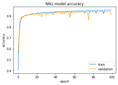
The plot above confirms that the model has converged on an optimal solution, with both training and validation accuracy increasing rapidly over the first 10 or so epochs and then flattening out after that. Not much further improvement in accuracy is obtained after the first 10 or so epochs.

Fit a convolutional neural network (CNN)

Next, a convolutional neural network (CNN) is constructed. CNNs are outlined in Section 5.7.1 of Module 5.

The CNN below will use two convolutional layers with a 5x5 filter/kernel.

cnn_model = Sequential()

cnn_model.add(Conv2D(filters = 16, kernel_size = (5,5), 
                 activation ='relu', input_shape = (28,28,1)))
  # Notice from the input_shape = (28,28,1) term above
  # that the CNN takes as input the 28x28 matrix of pixel features
  # rather than the flattened vector of all 784 pixel features. 
cnn_model.add(Conv2D(filters = 16, kernel_size = (5,5), 
                 activation ='relu'))
cnn_model.add(MaxPool2D(pool_size=(2,2)))

cnn_model.add(Flatten())
  # Flatten() converts the matrix outputs from the convolutional layers
  # back into vectors for feeding into the output layer. 
cnn_model.add(Dense(10, activation = 'softmax'))

# Define the regular stochastic gradient descent (SGD) optimiser (without
# momentum, a learning rate of 0.2 and the crossentropy loss function.
# to be used in the fitting of the model.
opt = SGD(learning_rate=0.2, momentum=0.0)
cnn_model.compile(optimizer = opt , loss = 'categorical_crossentropy',
                  metrics=['accuracy'])

epochs = 10
batch_size = 10

# Fit the CNN and capture the error and accuracy rates from the fitted model
# after each epoch.
cnn_hist = cnn_model.fit(train_cnn_x, train_y, batch_size = batch_size,
                         epochs = epochs,
                         validation_data = (validation_cnn_x, validation_y))

Epoch 1/10
2688/2688 [==============================] - 39s 14ms/step - loss: 0.5627 - accuracy: 0.8213 - val_loss: 0.1404 - val_accuracy: 0.9598
Epoch 2/10
2688/2688 [==============================] - 37s 14ms/step - loss: 1.4409 - accuracy: 0.4482 - val_loss: 2.3045 - val_accuracy: 0.1101
Epoch 3/10
2688/2688 [==============================] - 33s 12ms/step - loss: 2.3051 - accuracy: 0.1083 - val_loss: 2.3063 - val_accuracy: 0.1019
Epoch 4/10
2688/2688 [==============================] - 33s 12ms/step - loss: 2.3055 - accuracy: 0.1062 - val_loss: 2.3081 - val_accuracy: 0.1052
Epoch 5/10
2688/2688 [==============================] - 33s 12ms/step - loss: 2.3057 - accuracy: 0.1069 - val_loss: 2.3020 - val_accuracy: 0.1052
Epoch 6/10
2688/2688 [==============================] - 32s 12ms/step - loss: 2.3057 - accuracy: 0.1063 - val_loss: 2.3067 - val_accuracy: 0.1025
Epoch 7/10
2688/2688 [==============================] - 32s 12ms/step - loss: 2.3060 - accuracy: 0.1047 - val_loss: 2.3024 - val_accuracy: 0.1101
Epoch 8/10
2688/2688 [==============================] - 33s 12ms/step - loss: 2.3057 - accuracy: 0.1058 - val_loss: 2.3071 - val_accuracy: 0.0967
Epoch 9/10
2688/2688 [==============================] - 32s 12ms/step - loss: 2.3055 - accuracy: 0.1054 - val_loss: 2.3079 - val_accuracy: 0.1052
Epoch 10/10
2688/2688 [==============================] - 31s 11ms/step - loss: 2.3066 - accuracy: 0.1053 - val_loss: 2.3040 - val_accuracy: 0.1092

You should note that the CNN takes much longer to fit than the vanilla neural network (NN 1).

Evaluate CNN

# Plot the accuracy of the CNN against each epoch
# to ensure that the model has converged on an
# optimal solution.
plt.plot(cnn_hist.history['accuracy'],color='dodgerblue')
plt.plot(cnn_hist.history['val_accuracy'],color='orange')
plt.title('CNN model accuracy')
plt.ylabel('accuracy')
plt.xlabel('epoch')
plt.legend(['train', 'validation'], loc='lower right')

<matplotlib.legend.Legend at 0x158de8fd0>

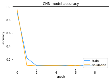
The graph of the accuracy suggests that the model may not have converged yet,since the validation accuracy is still volatile after 10 epochs. You can try to obtain a higher accuracy on the validation data by increasing the number of epochs used to train the model.

# Compare the accuracy obtained under the vanilla neural network (NN 1)
# to that obtained under the CNN.
{'CNN':cnn_hist.history['val_accuracy'][-1],
 'NN 1': nn_hist.history['val_accuracy'][-1]}

{'CNN': 0.10922618955373764, 'NN 1': 0.9074404835700989}

The CNN had a higher accuracy after 10 epochs compared to the vanilla neural network after 100 epochs. However, the CNN took substantially more time to train. The final choice of which model to use should take into account the business context and, in particular, the value that the business assigns to a model’s accuracy compared to its training efficiency.

Select the final model

# Select the final model and call it `nn_model_final`.
# In this case, it is assumed that model accuracy is
# more important than model training speed, hence the
# CNN is chosen.
nn_model_final = cnn_model
test_x_final = test_cnn_x

Observations

Predict on the test set

Now that a final fitted model has been selected, it can be used to make predictions on the test set.

# Make predictions on the test set.
test_preds = nn_model_final.predict(test_x_final)
# Convert the predictions (y_hat_gk) to class predictions (G(Xi.)).
test_preds_classes = np.argmax(test_preds,axis = 1)
# Convert the encoded responses (i.e. 0s and 1s to a single vector Numpy array
# contained classes 0, 1, 2, ..., 9.
test_y_classes = np.argmax(test_y,axis = 1)

Note that even though the CNN took a long time to train, it is very quick to score (i.e. make predictions based on a set of unseen observations).

# Use the confusion matrix function defined at the top of the notebook
# to observe the number of observations that have been
# misclassified by the final model.

# Compute the confusion matrix.
confusion_mtx = confusion_matrix(test_y_classes, test_preds_classes) 
# Plot the confusion matrix.
plot_confusion_matrix(confusion_mtx, classes = range(10))

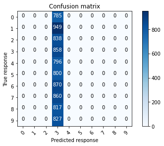
The confusion matrix above shows that the majority of observations have been correctly classified, as previously indicated by the high accuracy obtained from this model.

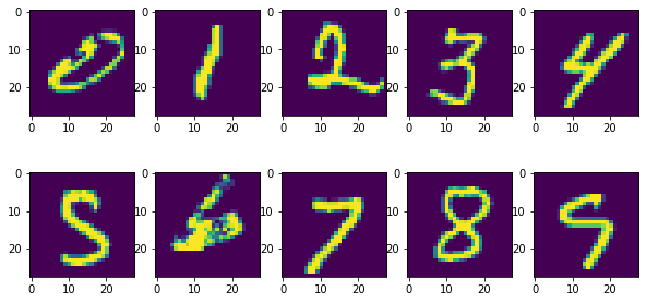
Observe example misclassifications

The code below allows you to observe some of the images that were misclassified by the final model. This information might be useful in working out particular types of images that the model found hard to classify correctly, which might inform how to further improve the model.

# Create a vector that allows errors to be identified.
errors = test_y_classes - test_preds_classes
error_indexes = np.where(errors != 0)

# Plot the first 10 errors.
fig = plt.figure(figsize=(10,5))
rows = 2
columns = 5
for i in range(0, 10):
    print(str(i+1)+'. Actual digit: ' + str(test_y_classes[error_indexes[0][i]]) +
          ' Predicted digit: ' + str(test_preds_classes[error_indexes[0][i]]))
    fig.add_subplot(rows, columns, i+1)
    plt.imshow(test_x_final[error_indexes[0][i]][:,:,0]);
plt.show()

1. Actual digit: 2 Predicted digit: 3
2. Actual digit: 2 Predicted digit: 3
3. Actual digit: 0 Predicted digit: 3
4. Actual digit: 9 Predicted digit: 3
5. Actual digit: 4 Predicted digit: 3
6. Actual digit: 6 Predicted digit: 3
7. Actual digit: 2 Predicted digit: 3
8. Actual digit: 9 Predicted digit: 3
9. Actual digit: 7 Predicted digit: 3
10. Actual digit: 0 Predicted digit: 3