Learn More

Learn More#

This content is from the Scientific Python QuickStart by Thomas J. Sargent and John Stachurski, originally published as the JupyterBook example. We will be gradually adding more introductory Python materials by actuarial contributors. In the meantime, consider also referring to the Python Study Group microsite for materials from the 2021 YDAWG-organised sessions.

We’re about ready to wrap up this brief course on Python for scientific computing.

In this last lecture we give some pointers to the major scientific libraries and suggestions for further reading.

NumPy#

Fundamental matrix and array processing capabilities are provided by the excellent NumPy library.

For example, let’s build some arrays

import numpy as np                     # Load the library

a = np.linspace(-np.pi, np.pi, 100)    # Create even grid from -π to π
b = np.cos(a)                          # Apply cosine to each element of a
c = np.sin(a)                          # Apply sin to each element of a

Now let’s take the inner product

b @ c

The number you see here might vary slightly due to floating point arithmetic but it’s essentially zero.

As with other standard NumPy operations, this inner product calls into highly optimized machine code.

It is as efficient as carefully hand-coded FORTRAN or C.

SciPy#

The SciPy library is built on top of NumPy and provides additional functionality.

For example, let’s calculate \(\int_{-2}^2 \phi(z) dz\) where \(\phi\) is the standard normal density.

from scipy.stats import norm
from scipy.integrate import quad

ϕ = norm()
value, error = quad(ϕ.pdf, -2, 2)  # Integrate using Gaussian quadrature
value

SciPy includes many of the standard routines used in

See them all here.

Graphics#

The most popular and comprehensive Python library for creating figures and graphs is Matplotlib, with functionality including

plots, histograms, contour images, 3D graphs, bar charts etc.
output in many formats (PDF, PNG, EPS, etc.)
LaTeX integration

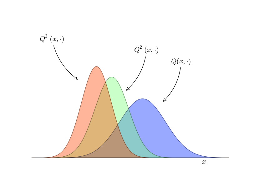
Example 2D plot with embedded LaTeX annotations

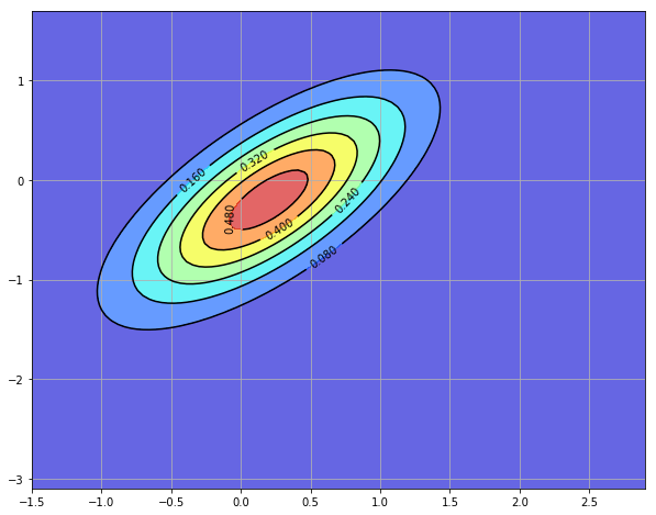
Example contour plot

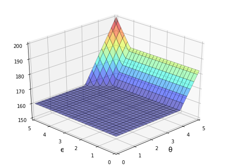
Example 3D plot

More examples can be found in the Matplotlib thumbnail gallery.

Other graphics libraries include

Plotly
Bokeh

Symbolic Algebra#

It’s useful to be able to manipulate symbolic expressions, as in Mathematica or Maple.

The SymPy library provides this functionality from within the Python shell.

from sympy import Symbol

x, y = Symbol('x'), Symbol('y')  # Treat 'x' and 'y' as algebraic symbols
x + x + x + y

We can manipulate expressions

expression = (x + y)**2
expression.expand()

solve polynomials

from sympy import solve

solve(x**2 + x + 2)

and calculate limits, derivatives and integrals

from sympy import limit, sin, diff

limit(1 / x, x, 0)

limit(sin(x) / x, x, 0)

diff(sin(x), x)

The beauty of importing this functionality into Python is that we are working within a fully fledged programming language.

We can easily create tables of derivatives, generate LaTeX output, add that output to figures and so on.

Pandas#

One of the most popular libraries for working with data is pandas.

Pandas is fast, efficient, flexible and well designed.

Here’s a simple example, using some dummy data generated with Numpy’s excellent random functionality.

import pandas as pd
np.random.seed(1234)

data = np.random.randn(5, 2)  # 5x2 matrix of N(0, 1) random draws
dates = pd.date_range('28/12/2010', periods=5)

df = pd.DataFrame(data, columns=('price', 'weight'), index=dates)
print(df)

df.mean()