Py: Socio-Economic Index Construction

This notebook was originally created by Andres Villegas Ramirez for the Data Analytics Applications subject, as Case study 1 - The Socio-Economic Indexes for Areas in the DAA M06 Unsupervised learning module.

Data Analytics Applications is a Fellowship Applications (Module 3) subject with the Actuaries Institute that aims to teach students how to apply a range of data analytics skills, such as neural networks, natural language processing, unsupervised learning and optimisation techniques, together with their professional judgement, to solve a variety of complex and challenging business problems. The business problems used as examples in this subject are drawn from a wide range of industries.

Find out more about the course here.

Purpose:

This case study demonstrates the use of principal component analysis (PCA) in the construction of an index to rank the socio-economic status of different geographical areas within a country (in this instance, Australia). Such index can be useful to identify areas that require funding or services, or as input for research into the relationship between socio-economic conditions and other outcomes in different areas.

In Australia, the Australian Bureau of Statistics (ABS) produces four of such indexes, referred to as the Socio-Economic Indexes for Areas (SEIFA). SEIFA ranks areas in Australia based on their relative socio-economic advantage and disadvantage.

This notebook replicates the methodology adopted by the ABS in constructing one of these indexes - Index of Economic Resources, or IER by Statistical Area 1 (SA1).

This Jupyter notebook is organised into the following sections:

• Section 1: Load required packages

• Section 2: Define a function for plotting

• Section 3: Import and transform data

• Section 4: Apply Principal Component Analysis and calibrate SEIFA score

• Section 5: Check against ABS publication

1. Load Packages

# Import required Python packages

#Dataframe operations
import pandas as pd 

#PCA
from sklearn.decomposition import PCA
from sklearn.preprocessing import StandardScaler

#Plotting
import matplotlib.pyplot as plt

2. Define Functions

# Define a function to obtain the explained variances from the PCA features.

## Good practice to define functions upfront.

def plot_explained_variances(pca):

    exp_var_pca = pca.explained_variance_ratio_

    plt.bar(range(1, len(exp_var_pca) + 1), exp_var_pca, alpha = 0.5, align = 'center',
            label='Individual explained variance',color='dodgerblue')
    plt.ylabel('Explained variance ratio')
    plt.xlabel('Principal component')
    plt.legend(loc='best')
    plt.tight_layout()
    plt.show()

3. Import and Transform Data

# Import data
## File 1: Standardised socio-economic variables published by the ABS (i.e. input to the PCA model)
## File 2: IER scores by Statistical Area 1 published by the ABS


infolder = 'https://actuariesinstitute.github.io/cookbook/_static/daa_datasets/'

file1 = 'standardised_variables_seifa_2021_cut.csv'
file2 = 'IER_2021.csv'

data1 = pd.read_csv(infolder + file1)
data2 = pd.read_csv(infolder + file2)

# Inspect data

## These are numerical features (e.g. % corresponding to a variable, see dictionary below) which are standardised

data1.head()

	SA1_2021	INC_LOW	INC_HIGH	ATSCHOOL	ATUNI	CERTIFICATE	DEGREE	DIPLOMA	NOYR12ORHIGHER	NOEDU	...	HIGHCAR	NOCAR	DISABILITYU70	ENGLISHPOOR	ONEPARENT	SEP_DIVORCED	UNINCORP	CHILDJOBLESS	MORTGAGEOVER30	RENTOVER30
0	10102100701	0.031160	-0.451226	-0.307998	-0.611843	2.110423	-0.792820	1.399224	0.039552	-0.494326	...	1.124942	-0.361674	1.160679	-0.628432	-0.087881	-0.046096	0.533110	-0.797863	0.427678	-1.208146
1	10102100702	-0.745478	0.235597	0.309750	-0.718416	0.795239	-0.138695	1.122862	-0.328068	-0.494326	...	2.165534	-0.737816	-1.371078	-0.628432	-1.513208	-0.216841	1.846095	-0.797863	0.322564	-1.208146
2	10102100703	0.207462	-0.333816	0.648522	-0.373289	0.143017	0.089753	-0.024178	-0.148292	-0.494326	...	-0.474119	-0.425240	-1.064640	-0.628432	0.078716	0.963607	0.486319	-0.335393	-0.486090	-0.029516
3	10102100704	0.383411	-0.417133	-1.082034	-0.887458	-0.308372	0.417513	-0.160872	0.083635	0.108973	...	-0.407742	-0.528653	0.038035	-0.628432	0.949299	1.482164	0.808398	0.554274	-0.156349	-0.423796
4	10102100705	0.334499	0.256282	-1.018268	-0.396676	0.235498	-0.072269	-0.227208	0.356362	-0.494326	...	-0.135464	-0.477578	0.056221	-0.628432	-1.048310	1.253986	0.795448	-0.116016	-0.297469	-0.292223

5 rows × 45 columns

Variable dictionary

Variable name	Variable description
INC_LOW	Per cent of people living in households with stated annual household equivalised income between \(1 and \)25,999 (approx. 1st and 2nd deciles)
LOWRENT	Per cent of occupied private dwellings paying rent less than \(250 per week (excluding \)0 per week)
NOCAR	Per cent of occupied private dwellings with no cars
LONE	Per cent of occupied private dwellings who are lone person occupied private dwellings
ONEPARENT	Per cent of one parent families with dependent offspring only
OVERCROWD	Per cent of occupied private dwellings requiring one or more extra bedrooms (based on Canadian National Occupancy Standard)
UNEMPLOYED_IER	Per cent of people aged 15 years and over who are unemployed
GROUP	Per cent of occupied private dwellings who are group occupied private dwellings
OWNING	Per cent of occupied private dwellings owning dwelling without a mortgage
UNINCORP	Per cent of dwellings with at least one person who is an owner of an unincorporated enterprise
INC_HIGH	Per cent of people with stated annual household equivalised income greater than $91,000
HIGHMORTGAGE	Per cent of occupied private dwellings paying mortgage greater than $2,800 per month
MORTGAGE	Per cent of occupied private dwellings owning dwelling (with a mortgage)
HIGHBED	Per cent of occupied private dwellings with four or more bedrooms

# Inspect data

## IER scored published based on 2021 Census data collection

data2.head()

	SA1_2021	IER_2021
0	10102100701	1023.037282
1	10102100702	1088.576036
2	10102100703	986.1022032
3	10102100704	965.4964701
4	10102100705	1013.432808

# Select variables ABS uses to calibrate the IER (per their methodology)

variable_IER = [
    'SA1_2021',
    'INC_LOW',
    'LOWRENT',
    'NOCAR',
    'LONE',
    'ONEPARENT',
    'OVERCROWD',
    'UNEMPLOYED_IER',
    'GROUP',
    'OWNING',
    'UNINCORP',
    'INC_HIGH',
    'HIGHMORTGAGE',
    'MORTGAGE',
    'HIGHBED'

]

data1_IER = data1[variable_IER]

# Inspect data type for these variables

data1_IER.info()

<class 'pandas.core.frame.DataFrame'>
RangeIndex: 59430 entries, 0 to 59429
Data columns (total 15 columns):
 #   Column          Non-Null Count  Dtype  
---  ------          --------------  -----  
 0   SA1_2021        59430 non-null  int64  
 1   INC_LOW         59427 non-null  float64
 2   LOWRENT         59400 non-null  float64
 3   NOCAR           59422 non-null  float64
 4   LONE            59430 non-null  float64
 5   ONEPARENT       59319 non-null  float64
 6   OVERCROWD       59417 non-null  float64
 7   UNEMPLOYED_IER  59429 non-null  float64
 8   GROUP           59430 non-null  float64
 9   OWNING          59423 non-null  float64
 10  UNINCORP        59430 non-null  float64
 11  INC_HIGH        59427 non-null  float64
 12  HIGHMORTGAGE    59400 non-null  float64
 13  MORTGAGE        59423 non-null  float64
 14  HIGHBED         59422 non-null  float64
dtypes: float64(14), int64(1)
memory usage: 6.8 MB

# Remove rows with missing values

print(data1_IER.isna().sum())
data1_IER_dropna = data1_IER.dropna()

SA1_2021            0
INC_LOW             3
LOWRENT            30
NOCAR               8
LONE                0
ONEPARENT         111
OVERCROWD          13
UNEMPLOYED_IER      1
GROUP               0
OWNING              7
UNINCORP            0
INC_HIGH            3
HIGHMORTGAGE       30
MORTGAGE            7
HIGHBED             8
dtype: int64

# Standardise data for PCA

## Select data from column 2 onwards (inclusive). First column is SA1 ID.
pca_data = data1_IER_dropna.iloc[:, 1:]

## Standardise these columns to mean 0 and variance 1
sc = StandardScaler()
sc.fit(pca_data)
pca_data = sc.transform(pca_data)

## Inspect outputs, each row represents a SA1 

print(data1_IER_dropna[50:55])
print(pca_data[50:55])

       SA1_2021   INC_LOW   LOWRENT     NOCAR      LONE  ONEPARENT  OVERCROWD  \
50  10102100921 -0.694978 -0.149470  0.026395  2.161618   0.016894   0.614584   
51  10102100923 -0.399570 -0.230663 -0.392438  0.346039   0.479932  -0.327006   
53  10102100925 -1.184584 -0.369694 -0.584525  1.995606   1.010923   0.163947   
54  10102100926 -0.755434  0.636737  0.194704  1.770099  -0.418760   0.828480   
55  10102100927 -0.534872 -0.113768 -0.443336 -0.248692  -0.929502   0.042116   

    UNEMPLOYED_IER     GROUP    OWNING  UNINCORP  INC_HIGH  HIGHMORTGAGE  \
50       -0.768433 -0.298797 -1.379936 -1.409706  0.565708     -0.711816   
51       -0.502225 -0.435782 -0.068099 -1.078581  0.417556     -0.309550   
53        0.393123  0.492720 -1.552475 -0.869567  0.401089     -0.914661   
54        0.562322  1.018832 -1.283807 -0.853606 -0.501616     -0.914661   
55       -0.591322  0.001803 -0.652794 -0.622710  0.248079      0.145029   

    MORTGAGE   HIGHBED  
50 -0.075949 -1.407022  
51  0.780225  0.198026  
53 -0.382142 -1.473097  
54 -1.468772 -1.443632  
55  0.547895  0.465557  
[[-6.97384349e-01 -1.49102654e-01  2.73842498e-02  2.18456511e+00
   1.68271418e-02  6.21443888e-01 -7.82538918e-01 -3.01193486e-01
  -1.38687638e+00 -1.42934823e+00  5.65712045e-01 -7.14208804e-01
  -8.01255787e-02 -1.41014150e+00]
 [-4.00578528e-01 -2.30600290e-01 -3.93807726e-01  3.52373086e-01
   4.80225191e-01 -3.29406608e-01 -5.11392783e-01 -4.39108873e-01
  -7.01834243e-02 -1.09373813e+00  4.17385805e-01 -3.11130864e-01
   7.79986710e-01  1.96337876e-01]
 [-1.18930828e+00 -3.70152778e-01 -5.86976088e-01  2.01703428e+00
   1.01162817e+00  1.66375413e-01  4.00564091e-01  4.95697733e-01
  -1.56005434e+00 -8.81893199e-01  4.00899556e-01 -9.17462999e-01
  -3.87727179e-01 -1.47627516e+00]
 [-7.58127412e-01  6.40055426e-01  1.96640397e-01  1.78946385e+00
  -4.19164718e-01  8.37443911e-01  5.72902051e-01  1.02538267e+00
  -1.29039226e+00 -8.65715951e-01 -5.02866086e-01 -9.17462999e-01
  -1.47935650e+00 -1.44678433e+00]
 [-5.36520854e-01 -1.13266264e-01 -4.44992083e-01 -2.47800227e-01
  -9.30303140e-01  4.33461879e-02 -6.02142493e-01  1.44766450e-03
  -6.57042865e-01 -6.31693191e-01  2.47710087e-01  1.44364950e-01
   5.46588117e-01  4.64107182e-01]]

4. Modelling

This section performs the PCA to recreate the ABS’s IER Index.

# Initiate the PCA.
pca = PCA()

# Fit the PCA model to determine the transformed features.
## It took 2 lines to fit the PCA model.
pca.fit_transform(pca_data)

# Plot variance explained by principal components
plot_explained_variances(pca)

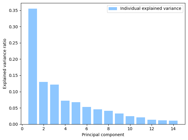
Principal component 1 (PC1) explains over 30% of the variance in the data. PC1 is used as the basis of calculating the IER.

pca_data[0]

array([ 3.21902216e-02, -1.95351071e-01, -3.62869762e-01,  3.59364682e-01,
       -8.80285299e-02,  1.99924572e-01, -6.52078395e-01, -9.12914962e-01,
        1.26794033e+00,  5.39782081e-01, -4.52416487e-01, -3.17209382e-01,
        2.45495526e-01,  4.39423025e-04])

# Reverse sign (per ABS methodology)

pca_data_transformed = -1.0*pca.fit_transform(pca_data)

# Extract first principal component in a dataframe
pca1 = pd.DataFrame(pca_data_transformed[:, 0], columns = ['IER_2021'])

# Attach SA1 ID to
IER_S1 = pd.concat([data1_IER_dropna['SA1_2021'].reset_index(drop = True), pca1]
                    , axis=1)

print(IER_S1.head(1))

      SA1_2021  IER_2021
0  10102100701  0.517295

# Calculation from first principal
## Sign implies how each variable contributes to a score
## Reverse sign to make it more comprehensive

component_df = pd.DataFrame({
    'Variable': data1_IER.columns[1:],
    'PC1 Loading': -1.0 * pca.components_[0],
    'First SA1': pca_data[0]
})

print(component_df)


raw_score_first_SA1 = (component_df['PC1 Loading'] * component_df['First SA1']).sum()


print('\n')
print('\n')
print(raw_score_first_SA1)

          Variable  PC1 Loading  First SA1
0          INC_LOW    -0.327920   0.032190
1          LOWRENT    -0.320014  -0.195351
2            NOCAR    -0.316516  -0.362870
3             LONE    -0.307799   0.359365
4        ONEPARENT    -0.243785  -0.088029
5        OVERCROWD    -0.231555   0.199925
6   UNEMPLOYED_IER    -0.217694  -0.652078
7            GROUP    -0.175738  -0.912915
8           OWNING     0.152087   1.267940
9         UNINCORP     0.211586   0.539782
10        INC_HIGH     0.233597  -0.452416
11    HIGHMORTGAGE     0.285636  -0.317209
12        MORTGAGE     0.295868   0.245496
13         HIGHBED     0.334995   0.000439




0.5172947202278048

A recap of the dataframe operations for transforming raw data to principal components

Dataframe name	Operations
data1	Raw data we’ll be using to replicate the SEIFA IER score, numercial features (%)
data1_IER	Select features for determining IER from data1
data1_IER_dropna	Remove missing values in data1_IER
pca_data	Standardise features in data1_IER_dropna to mean 0 and s.d. 1, used to perform PCA
pca	Output of PCA, Principal Components
pca_data_transformed	Reverse sign in pca
pca1	Extract first principal component from pca_data_transformed
IER_S1	Attach SA1 identifier to pca1, compared to dataframe ABS_IER_S1 which is the published data

# Standardise calibrated IER scores to mean of 1,000 and standard deviation of 100 (per ABS methodology)

IER_S1['IER_recreated'] = (IER_S1['IER_2021']/IER_S1['IER_2021'].std())*100+1000

print(IER_S1.tail())

          SA1_2021  IER_2021  IER_recreated
59298  90104100401  0.022187    1000.995399
59299  90104100402 -0.055935     997.490510
59300  90104100403 -0.785740     964.748521
59301  90104100404 -1.702813     923.604956
59302  90104100407 -0.116936     994.753789

5. Reconcile with ABS publication

# Extract first two columns in the desired data type

ABS_IER_S1 = data2.iloc[:, [0, 1]]

ABS_IER_S1['IER_2021'] = pd.to_numeric(ABS_IER_S1['IER_2021'],
                                        errors='coerce')
ABS_IER_S1['SA1_2021'] = pd.to_numeric(ABS_IER_S1['SA1_2021'],
                                        errors='coerce', downcast = 'integer')


print(ABS_IER_S1.info())
print('\n')
print(ABS_IER_S1.head())
print('\n')
print(ABS_IER_S1.isna().sum())

<class 'pandas.core.frame.DataFrame'>
RangeIndex: 59421 entries, 0 to 59420
Data columns (total 2 columns):
 #   Column    Non-Null Count  Dtype  
---  ------    --------------  -----  
 0   SA1_2021  59421 non-null  int64  
 1   IER_2021  59303 non-null  float64
dtypes: float64(1), int64(1)
memory usage: 928.6 KB
None


      SA1_2021     IER_2021
0  10102100701  1023.037282
1  10102100702  1088.576036
2  10102100703   986.102203
3  10102100704   965.496470
4  10102100705  1013.432808


SA1_2021      0
IER_2021    118
dtype: int64

## Remove rows with missing value

print(ABS_IER_S1.isna().sum())
ABS_IER_S1_dropna = ABS_IER_S1.dropna()

print(len(data1_IER_dropna))
print(len(ABS_IER_S1_dropna))

SA1_2021      0
IER_2021    118
dtype: int64
59303
59303

# Merge the recreated with the published data for reconciliation 1 - histograms

join = pd.merge(ABS_IER_S1_dropna, data1_IER_dropna, how = 'left', on = 'SA1_2021')

# Plot histogram of calibrated IER scores

IER_S1.hist(column='IER_recreated', bins=100, color='dodgerblue')
plt.title('Distribution of recreated IER scores')
plt.xlabel('IER score')
plt.ylabel('Frequency')

plt.show()

# Plot histogram of publisehd IER scores

ABS_IER_S1_dropna.hist(column='IER_2021', bins=100, color='dodgerblue')
plt.title('Distribution of ABS IER scores')
plt.xlabel('IER score')
plt.ylabel('Frequency')

plt.show()

ABS_IER_S1_dropna.to_csv('check_ABS_IER_S1_dropna.csv')

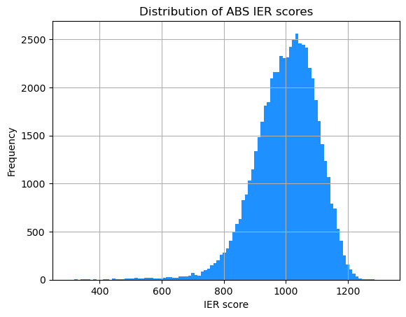
The two histograms are very similar in shape!

# Extract columns we need

IER_S1_reduce = IER_S1[['SA1_2021', 'IER_recreated']]

# Merge the recreated with the published data for reconciliation 2 - scatter plot

IER_join = pd.merge(ABS_IER_S1_dropna, IER_S1_reduce, how = 'left', on = 'SA1_2021')

print(IER_join.tail())

          SA1_2021     IER_2021  IER_recreated
59298  90104100401  1000.369129    1000.995399
59299  90104100402   996.979765     997.490510
59300  90104100403   964.139169     964.748521
59301  90104100404   923.050144     923.604956
59302  90104100407   994.377312     994.753789

# Plot calibrated score vs. published score

plt.scatter('IER_recreated', 'IER_2021', data = IER_join, color='dodgerblue')
plt.title('Comparison of recreated and ABS IER scores')
plt.xlabel('Recreated IER score')
plt.ylabel('ABS IER score')

plt.show()

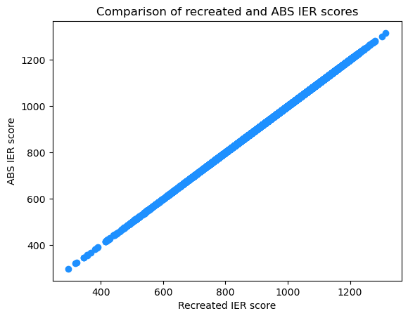
The above scatter plot shows that the two sets of indexes are very closely aligned.