R: Life Industry Stats in Tableau and R#
By Pat Reen - originally published on his GitHub site here, which has the original code.
Overview#
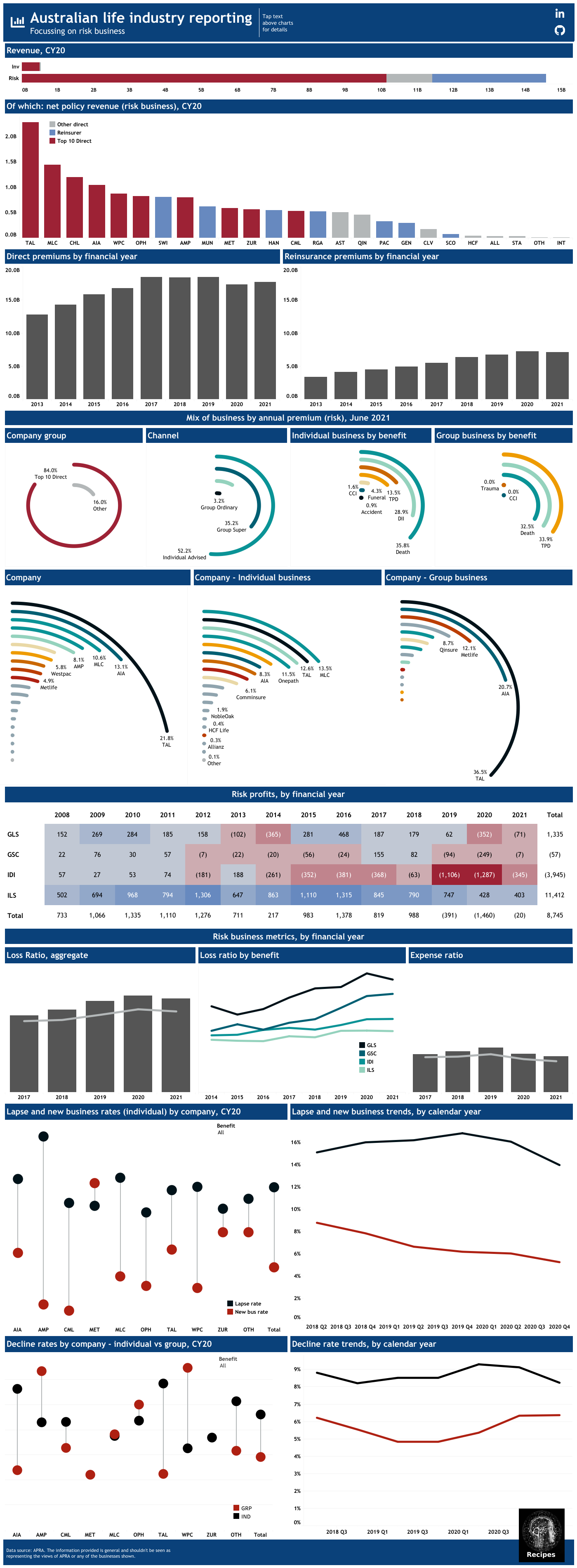
APRA release Australian life industry data on performance quarterly at a product level as well as aggregated results by company. Bi-annually APRA release other statistics on lapse rates, new business rates, decline rates and market share. This section presents a visualisation of these datasources in Tableau. Also included is an R script which could be used to extract results from the APRA data.
Tableau public is a free to use visualisation tool that can ingest data in a number of different formats and is useful at creating flexible visualisation.
See link above to GitHub repository which has data and tableau workbook for this recipe.
Introducing radial bar charts#
A radial bar chart is a bar chart plotted in polar co-ordinates rather than a Cartesian plane. This site sets out a very simple approach, which are used here.
The result#
A preview of the final visualisation is below (click through to Tableau):
Using r to view industry stats#
As with most data sources, an alternative visualisation tool is R. The below extracts the individual disability income profits and revenue and calculates the margin.
not_run_sample_only <- function(){
# this script reads in the APRA data and produces a few graphs for presentation

packages <- c("tidyverse", "ggplot2", "readxl", "lubridate", "scales", "xtable")
install.packages(setdiff(packages, rownames(installed.packages())))
for (package in packages) {
    library(package, character.only = TRUE)
}

percent0 <- function(value) {
  return(percent(value, accuracy = 0.1))
}

# update names
# [1] "Reporting date"      "Industry sector"     "Subject"
# [4] "Category"            "Data item"           "Reporting Structure"
# [7] "Class of business"   "Product Group"       "Calculation basis"
# [10] "Value"               "Notes"

qrt_col_name <- c(
  "rep_date", "sector", "subject", "category", "data_item",
  "rep_struc", "class", "product", "calc_basis", "value",
  "notes"
)
qrt_col_type <- c("date", rep("text", 8), "numeric", "text")

#---------- read in quarterly data
qrt_data <- read_xlsx(
# update to relevant path
  path = "Quarterly life insurance performance statistics database - June 2008 to June 2021.xlsx",
  sheet = "Data",
  col_names = qrt_col_name,
  skip = 1,
  col_types = qrt_col_type,
  trim_ws = TRUE, na = "N/A"
)

# add fiscal years
qrt_data$fin_year <- paste0("FY", format(year(qrt_data$rep_date) +
  as.integer(month(qrt_data$rep_date) > 6)))
# also add calendar year as an alternative aggregation
qrt_data$cal_year <- format(year(qrt_data$rep_date))


# DI Profit by Year -----------------------------------------------------

DI_risk_type <- "Individual Disability Income Insurance"

data_items <- c(
    "Profit / loss before tax ($m)" = "Profit / loss before tax",
    "Premiums after reinsurance ($m)" = "Net policy revenue",
    "Premiums before reinsurance ($m)" = "Gross policy revenue"
)

DI_profit <- qrt_data %>%
  filter(data_item %in% data_items) %>%
  filter(is.na(class)) %>%
  filter(product == DI_risk_type) %>%
  group_by(`Fin year` = fin_year, data_item) %>%
  summarise(risk_value = sum(value)) %>%
  spread(data_item, risk_value) %>%
  mutate(`Margin (%)` = percent0(`Profit / loss before tax` /
  `Net policy revenue`)) %>%
  rename(data_items)

DI_profit_print <- xtable(
    x = DI_profit,
    caption = "Individual Disability Income Industry Profit",
    align = "llrrrr",
    digits = 0
)

print(DI_profit_print,
      type = "html",
      file = "DI_profit",
      include.rownames = FALSE,
      )
}