R: Baudry ML Reserving Pt 1#
This article was originally created by Nigel Carpenter and published in the General Insurance Machine Learning for Reserving Working Party (“MLR-WP”) blog. The MLR-WP is an international research group on machine learning techniques to reserving, with over 50 actuaries from around the globe. The goal of the group is to bring machine learning techniques into widespread adoption ‘on the ground’ by identifying what the barriers are, communicating any benefits, and helping develop the research techniques in pragmatic ways. Whilst some articles have been brought into this cookbook, consider exploring the blog further for additional content including detailed walkthroughs of more advanced models.
Introduction#
This is the first notebook of a series of three that outlines and elaborates upon code used to replicate the central scenario in the paper of Maximilien Baudry “NON-PARAMETRIC INDIVIDUAL CLAIM RESERVING IN INSURANCE” (Presentation Paper)
Below we step through the process to create a single simulated dataset, as set out in Section 5 of Baudry’s paper. Having stepped through the data creation process, at the end, we present the code in the form of a function that returns a simulated policy and claim dataset.
The second notebook details the process for creating a reserving database and the third outlines the process for creating reserves using machine learning.
Before we start we import a few pre-requisite R packages.
# Importing packages
library(data.table)
library(magrittr)
library(lubridate)
library(ggplot2)
library(cowplot)
library(repr)
library(kableExtra)
library(IRdisplay)
Attaching package: ‘lubridate’


The following objects are masked from ‘package:data.table’:

    hour, isoweek, mday, minute, month, quarter, second, wday, week,
    yday, year


The following objects are masked from ‘package:base’:

    date, intersect, setdiff, union


Attaching package: ‘cowplot’


The following object is masked from ‘package:lubridate’:

    stamp
Create Policy Data set#
We start by simulating number of policies sold by day and by policy coverage type.
Policy count by date#
# polices sold between start 2016 to end 2017
dt_policydates <- data.table(date_UW = seq(as.Date("2016/1/1"), as.Date("2017/12/31"), "day"))

# number of policies per day follows Poisson process with mean 700 (approx 255,500 pols per annum)
dt_policydates[, ':='(policycount = rpois(.N,700),
                      date_lapse = date_UW %m+% years(1),
                      expodays = as.integer(date_UW %m+% years(1) - date_UW),
                      pol_prefix = year(date_UW)*10000 + month(date_UW)*100 + mday(date_UW))]
Policy covers by date#
We then add policy coverage columns in proportions 25% Breakage, 45% Breakage and Oxidation and 30% Breakage, Oxidation and Theft.
# Add columns defining Policy Covers
dt_policydates[, Cover_B := round(policycount * 0.25)]
dt_policydates[, Cover_BO := round(policycount * 0.45)]
dt_policydates[, Cover_BOT := policycount - Cover_B - Cover_BO]
kable(head(dt_policydates), "html") %>%
  kable_styling("striped") %>%
  scroll_box(width = "100%") %>%
  as.character() %>%
  display_html()
| date_UW | policycount | date_lapse | expodays | pol_prefix | Cover_B | Cover_BO | Cover_BOT |
|---|---|---|---|---|---|---|---|
| 2016-01-01 | 693 | 2017-01-01 | 366 | 20160101 | 173 | 312 | 208 |
| 2016-01-02 | 690 | 2017-01-02 | 366 | 20160102 | 172 | 310 | 208 |
| 2016-01-03 | 716 | 2017-01-03 | 366 | 20160103 | 179 | 322 | 215 |
| 2016-01-04 | 714 | 2017-01-04 | 366 | 20160104 | 178 | 321 | 215 |
| 2016-01-05 | 727 | 2017-01-05 | 366 | 20160105 | 182 | 327 | 218 |
| 2016-01-06 | 763 | 2017-01-06 | 366 | 20160106 | 191 | 343 | 229 |
Policy transaction file#
We then create a policy transaction file containing 1 row per policy, with columns to indicate policy coverage details.
Policy date & number#
The first step is to create a policy table with 1 row per policy and underwriting date.
# repeat rows for each policy by UW-Date
dt_policy <- dt_policydates[rep(1:.N, policycount),c("date_UW", "pol_prefix"), with = FALSE][,pol_seq:=1:.N, by=pol_prefix]

# Create a unique policy number
dt_policy[, pol_number := as.character(pol_prefix * 10000 + pol_seq)]

kable(head(dt_policy), "html") %>%
  kable_styling("striped") %>%
  scroll_box(width = "100%") %>%
  as.character() %>%
  display_html()
| date_UW | pol_prefix | pol_seq | pol_number |
|---|---|---|---|
| 2016-01-01 | 20160101 | 1 | 201601010001 |
| 2016-01-01 | 20160101 | 2 | 201601010002 |
| 2016-01-01 | 20160101 | 3 | 201601010003 |
| 2016-01-01 | 20160101 | 4 | 201601010004 |
| 2016-01-01 | 20160101 | 5 | 201601010005 |
| 2016-01-01 | 20160101 | 6 | 201601010006 |
Policy coverage type#
Then we add the policy coverage details appropriate to each row.
# set join keys
setkey(dt_policy,'date_UW')
setkey(dt_policydates,'date_UW')

# remove pol_prefix before join
dt_policydates[, pol_prefix := NULL]

# join cover from summary file (dt_policydates)
dt_policy <- dt_policy[dt_policydates]

# now create Cover field for each policy row
dt_policy[,Cover := 'BO']
dt_policy[pol_seq <= policycount- Cover_BO,Cover := 'BOT']
dt_policy[pol_seq <= Cover_B,Cover := 'B']

dt_policy[, Cover_B := as.factor(Cover)]

# remove interim calculation fields
dt_policy[, ':='(pol_prefix = NULL,
                 policycount = NULL,
                 pol_seq = NULL,
                 Cover_B = NULL,
                 Cover_BOT = NULL,
                 Cover_BO = NULL)]

# check output
kable(head(dt_policy), "html") %>%
  kable_styling("striped") %>%
  scroll_box(width = "100%") %>%
  as.character() %>%
  display_html()
| date_UW | pol_number | date_lapse | expodays | Cover |
|---|---|---|---|---|
| 2016-01-01 | 201601010001 | 2017-01-01 | 366 | B |
| 2016-01-01 | 201601010002 | 2017-01-01 | 366 | B |
| 2016-01-01 | 201601010003 | 2017-01-01 | 366 | B |
| 2016-01-01 | 201601010004 | 2017-01-01 | 366 | B |
| 2016-01-01 | 201601010005 | 2017-01-01 | 366 | B |
| 2016-01-01 | 201601010006 | 2017-01-01 | 366 | B |
Policy Brand, Price, Model features#
Now further details can be added to the policy dataset; such as policy brand, model and price details.
# Add remaining policy details
dt_policy[, Brand := rep(rep(c(1,2,3,4), c(9,6,3,2)), length.out = .N)]
dt_policy[, Base_Price := rep(rep(c(600,550,300,150), c(9,6,3,2)), length.out = .N)]

# models types and model cost multipliers
for (eachBrand in unique(dt_policy$Brand)) {
  dt_policy[Brand == eachBrand, Model := rep(rep(c(3,2,1,0), c(10, 7, 2, 1)), length.out = .N)]
  dt_policy[Brand == eachBrand, Model_mult := rep(rep(c(1.15^3, 1.15^2, 1.15^1, 1.15^0), c(10, 7, 2, 1)), length.out = .N)]
}

dt_policy[, Price := ceiling (Base_Price * Model_mult)]

# check output
kable(head(dt_policy), "html") %>%
  kable_styling("striped") %>%
  scroll_box(width = "100%") %>%
  as.character() %>%
  display_html()
| date_UW | pol_number | date_lapse | expodays | Cover | Brand | Base_Price | Model | Model_mult | Price |
|---|---|---|---|---|---|---|---|---|---|
| 2016-01-01 | 201601010001 | 2017-01-01 | 366 | B | 1 | 600 | 3 | 1.520875 | 913 |
| 2016-01-01 | 201601010002 | 2017-01-01 | 366 | B | 1 | 600 | 3 | 1.520875 | 913 |
| 2016-01-01 | 201601010003 | 2017-01-01 | 366 | B | 1 | 600 | 3 | 1.520875 | 913 |
| 2016-01-01 | 201601010004 | 2017-01-01 | 366 | B | 1 | 600 | 3 | 1.520875 | 913 |
| 2016-01-01 | 201601010005 | 2017-01-01 | 366 | B | 1 | 600 | 3 | 1.520875 | 913 |
| 2016-01-01 | 201601010006 | 2017-01-01 | 366 | B | 1 | 600 | 3 | 1.520875 | 913 |
Tidy and save#
The final step is to keep only columns of interest and save the resulting policy file.
# colums to keep
cols_policy <- c("pol_number",
                 "date_UW",
                 "date_lapse",
                 "Cover",
                 "Brand",
                 "Model",
                 "Price")

dt_policy <- dt_policy[, cols_policy, with = FALSE]

# check output
kable(head(dt_policy), "html") %>%
  kable_styling("striped") %>%
  scroll_box(width = "100%") %>%
  as.character() %>%
  display_html()

save(dt_policy, file = "./dt_policy.rda")
| pol_number | date_UW | date_lapse | Cover | Brand | Model | Price |
|---|---|---|---|---|---|---|
| 201601010001 | 2016-01-01 | 2017-01-01 | B | 1 | 3 | 913 |
| 201601010002 | 2016-01-01 | 2017-01-01 | B | 1 | 3 | 913 |
| 201601010003 | 2016-01-01 | 2017-01-01 | B | 1 | 3 | 913 |
| 201601010004 | 2016-01-01 | 2017-01-01 | B | 1 | 3 | 913 |
| 201601010005 | 2016-01-01 | 2017-01-01 | B | 1 | 3 | 913 |
| 201601010006 | 2016-01-01 | 2017-01-01 | B | 1 | 3 | 913 |
Create claims file#
Sample Claims from Policies#
We now simulate claims arising from the policy coverages. Claim rates vary by policy coverage and type.
Breakage Claims#
We start with breakages claims and sample from the policies data set to create claims.
# All policies have breakage cover
# claims uniformly sampled from policies
claim <- sample(nrow(dt_policy), size = floor(nrow(dt_policy) * 0.15))

# Claim severity multiplier sampled from beta distribution
dt_claim <- data.table(pol_number = dt_policy[claim, pol_number],
                       claim_type = 'B',
                       claim_count = 1,
                       claim_sev = rbeta(length(claim), 2,5))

# check output
kable(head(dt_claim), "html") %>%
  kable_styling("striped") %>%
  scroll_box(width = "100%") %>%
  as.character() %>%
  display_html()
| pol_number | claim_type | claim_count | claim_sev |
|---|---|---|---|
| 201706250197 | B | 1 | 0.0066006 |
| 201702160566 | B | 1 | 0.1305747 |
| 201703080185 | B | 1 | 0.3325863 |
| 201709090113 | B | 1 | 0.2690556 |
| 201604260297 | B | 1 | 0.2531805 |
| 201707310143 | B | 1 | 0.1357897 |
Oxidation Claims#
Oxidation claims follow a similar process, just with different incidence rates and severities.
# identify all policies with Oxidation cover
cov <- which(dt_policy$Cover != 'B')

# sample claims from policies with cover
claim <- sample(cov, size = floor(length(cov) * 0.05))

# add claims to table
dt_claim <- rbind(dt_claim,
                  data.table(pol_number = dt_policy[claim, pol_number],
                             claim_type = 'O',
                             claim_count = 1,
                             claim_sev = rbeta(length(claim), 5,3)))

# check output
kable(head(dt_claim), "html") %>%
  kable_styling("striped") %>%
  scroll_box(width = "100%") %>%
  as.character() %>%
  display_html()
| pol_number | claim_type | claim_count | claim_sev |
|---|---|---|---|
| 201706250197 | B | 1 | 0.0066006 |
| 201702160566 | B | 1 | 0.1305747 |
| 201703080185 | B | 1 | 0.3325863 |
| 201709090113 | B | 1 | 0.2690556 |
| 201604260297 | B | 1 | 0.2531805 |
| 201707310143 | B | 1 | 0.1357897 |
Theft Claims#
In the original paper the distribution for Theft severity claims is stated to be Beta(alpha = 5, beta = 0.5).
# identify all policies with Theft cover
# for Theft claim frequency varies by Brand
# So need to consider each in turn...

for(myModel in 0:3) {

    cov <- which(dt_policy$Cover == 'BOT' & dt_policy$Model == myModel)
    claim <- sample(cov, size = floor(length(cov) * 0.05*(1 + myModel)))

    dt_claim <- rbind(dt_claim,
                      data.table(pol_number = dt_policy[claim, pol_number],
                                 claim_type = 'T',
                                 claim_count = 1,
                                 claim_sev = rbeta(length(claim), 5,.5)))
}

# check output
kable(head(dt_claim), "html") %>%
  kable_styling("striped") %>%
  scroll_box(width = "100%") %>%
  as.character() %>%
  display_html()

kable(tail(dt_claim), "html") %>%
  kable_styling("striped") %>%
  scroll_box(width = "100%") %>%
  as.character() %>%
  display_html()
| pol_number | claim_type | claim_count | claim_sev |
|---|---|---|---|
| 201706250197 | B | 1 | 0.0066006 |
| 201702160566 | B | 1 | 0.1305747 |
| 201703080185 | B | 1 | 0.3325863 |
| 201709090113 | B | 1 | 0.2690556 |
| 201604260297 | B | 1 | 0.2531805 |
| 201707310143 | B | 1 | 0.1357897 |
| pol_number | claim_type | claim_count | claim_sev |
|---|---|---|---|
| 201708230205 | T | 1 | 0.9648917 |
| 201701280297 | T | 1 | 0.8245351 |
| 201701020337 | T | 1 | 0.7794176 |
| 201605080388 | T | 1 | 0.8335502 |
| 201608140365 | T | 1 | 0.9262032 |
| 201710040235 | T | 1 | 0.6904011 |
Claim dates and costs#
Policy UW_date and value#
We now need to add details to claims, such as policy underwritng date and phone cost. These details come from the policy table.
# set join keys
setkey(dt_policy, pol_number)
setkey(dt_claim, pol_number)

#join Brand and Price from policy to claim
dt_claim[dt_policy,
         on = 'pol_number',
         ':='(date_UW = i.date_UW,
              Price = i.Price,
              Brand = i.Brand)]

# check output
kable(head(dt_claim), "html") %>%
  kable_styling("striped") %>%
  scroll_box(width = "100%") %>%
  as.character() %>%
  display_html()
| pol_number | claim_type | claim_count | claim_sev | date_UW | Price | Brand |
|---|---|---|---|---|---|---|
| 201601010003 | B | 1 | 0.2786004 | 2016-01-01 | 913 | 1 |
| 201601010019 | B | 1 | 0.3383702 | 2016-01-01 | 229 | 4 |
| 201601010021 | B | 1 | 0.2924503 | 2016-01-01 | 913 | 1 |
| 201601010028 | B | 1 | 0.2193067 | 2016-01-01 | 794 | 1 |
| 201601010032 | B | 1 | 0.2106113 | 2016-01-01 | 837 | 2 |
| 201601010047 | B | 1 | 0.1108387 | 2016-01-01 | 913 | 1 |
Add simulated Claim occrrence, reporting and payment delays#
The occurrence delay is assumed uniform over policy exposure period. Reporting and payment delays are assumed to follow Beta distributions.
# use lubridate %m+% date addition operator
dt_claim[, date_lapse := date_UW %m+% years(1)]
dt_claim[, expodays := as.integer(date_lapse - date_UW)]
dt_claim[, occ_delay_days := floor(expodays * runif(.N, 0,1))]

dt_claim[ ,delay_report := floor(365 * rbeta(.N, .4, 10))]
dt_claim[ ,delay_pay := floor(10 + 40* rbeta(.N, 7,7))]

dt_claim[, date_occur := date_UW %m+% days(occ_delay_days)]
dt_claim[, date_report := date_occur %m+% days(delay_report)]
dt_claim[, date_pay := date_report %m+% days(delay_pay)]

dt_claim[, claim_cost := round(Price * claim_sev)]
# check output
head(dt_claim)
| pol_number | claim_type | claim_count | claim_sev | date_UW | Price | Brand | date_lapse | expodays | occ_delay_days | delay_report | delay_pay | date_occur | date_report | date_pay | claim_cost |
|---|---|---|---|---|---|---|---|---|---|---|---|---|---|---|---|
| <chr> | <chr> | <dbl> | <dbl> | <date> | <dbl> | <dbl> | <date> | <int> | <dbl> | <dbl> | <dbl> | <date> | <date> | <date> | <dbl> |
| 201601010003 | B | 1 | 0.2786004 | 2016-01-01 | 913 | 1 | 2017-01-01 | 366 | 173 | 71 | 28 | 2016-06-22 | 2016-09-01 | 2016-09-29 | 254 |
| 201601010019 | B | 1 | 0.3383702 | 2016-01-01 | 229 | 4 | 2017-01-01 | 366 | 139 | 6 | 33 | 2016-05-19 | 2016-05-25 | 2016-06-27 | 77 |
| 201601010021 | B | 1 | 0.2924503 | 2016-01-01 | 913 | 1 | 2017-01-01 | 366 | 203 | 2 | 30 | 2016-07-22 | 2016-07-24 | 2016-08-23 | 267 |
| 201601010028 | B | 1 | 0.2193067 | 2016-01-01 | 794 | 1 | 2017-01-01 | 366 | 186 | 1 | 29 | 2016-07-05 | 2016-07-06 | 2016-08-04 | 174 |
| 201601010032 | B | 1 | 0.2106113 | 2016-01-01 | 837 | 2 | 2017-01-01 | 366 | 199 | 33 | 29 | 2016-07-18 | 2016-08-20 | 2016-09-18 | 176 |
| 201601010047 | B | 1 | 0.1108387 | 2016-01-01 | 913 | 1 | 2017-01-01 | 366 | 141 | 0 | 29 | 2016-05-21 | 2016-05-21 | 2016-06-19 | 101 |
Claim key and tidy#
The final stage is to do some simple tidying and add a unique claim key. The file is then saved for future use.
Note that the original paper spoke of using a “competing hazards model” for simulating claims. I have taken this to mean that a policy can only give rise to one claim. Where the above process has simulated multiple claims against the same policy I keep only the first occurring claim.
# add a unique claimkey based upon occurence date

dt_claim[, clm_prefix := year(date_occur)*10000 + month(date_occur)*100 + mday(date_occur)]
dt_claim[, clm_seq := seq_len(.N), by = clm_prefix]
dt_claim[, clm_number := as.character(clm_prefix * 10000 + clm_seq)]


# keep only first claim against policy (competing hazards)
setkeyv(dt_claim, c("pol_number", "clm_prefix"))
dt_claim[, polclm_seq := seq_len(.N), by = .(pol_number)]
dt_claim <- dt_claim[polclm_seq == 1,]

# colums to keep
cols_claim <- c("clm_number",
                "pol_number",
                "claim_type",
                "claim_count",
                "claim_sev",
                "date_occur",
                "date_report",
                "date_pay",
                "claim_cost")

dt_claim <- dt_claim[, cols_claim, with = FALSE]

# check output
kable(head(dt_claim), "html") %>%
  kable_styling("striped") %>%
  scroll_box(width = "100%") %>%
  as.character() %>%
  display_html()

save(dt_claim, file = "./dt_claim.rda")
| clm_number | pol_number | claim_type | claim_count | claim_sev | date_occur | date_report | date_pay | claim_cost |
|---|---|---|---|---|---|---|---|---|
| 201606220001 | 201601010003 | B | 1 | 0.2786004 | 2016-06-22 | 2016-09-01 | 2016-09-29 | 254 |
| 201605190001 | 201601010019 | B | 1 | 0.3383702 | 2016-05-19 | 2016-05-25 | 2016-06-27 | 77 |
| 201607220001 | 201601010021 | B | 1 | 0.2924503 | 2016-07-22 | 2016-07-24 | 2016-08-23 | 267 |
| 201607050001 | 201601010028 | B | 1 | 0.2193067 | 2016-07-05 | 2016-07-06 | 2016-08-04 | 174 |
| 201607180001 | 201601010032 | B | 1 | 0.2106113 | 2016-07-18 | 2016-08-20 | 2016-09-18 | 176 |
| 201605210001 | 201601010047 | B | 1 | 0.1108387 | 2016-05-21 | 2016-05-21 | 2016-06-19 | 101 |
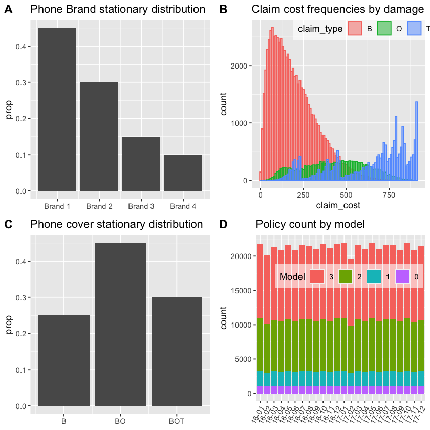
Checking exhibits#
Baudry’s paper produced a number of summary exhibits from the simulated data. Let’s recreate them to get some comfort that we have correctly recreated the data.
You can see that the severity exhibit, Chart B, is inconsistent with that presented in the original paper. The cause of that difference is unclear at the time of writing. It’s likely to be because something nearer to a Beta(alpha = 5, beta = 0.05) has been used. However using that creates other discrepancies likely to be due to issues with the competing hazards implementation. For now we note the differences and continue with the data as created here.
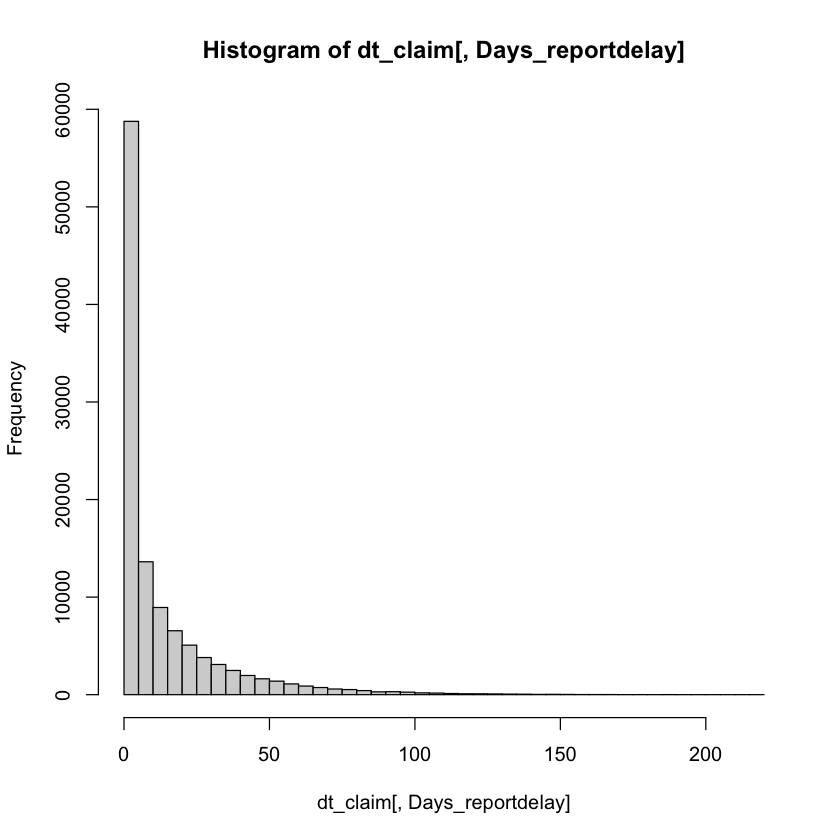
dt_claim[, Days_reportdelay := as.numeric(difftime(date_report, date_occur, units="days"))]


hist(dt_claim[, Days_reportdelay],breaks = 50)
dt_claim[, Days_paymentdelay := as.numeric(difftime(date_pay, date_report, units="days"))]
hist(dt_claim[, Days_paymentdelay],breaks = 60)

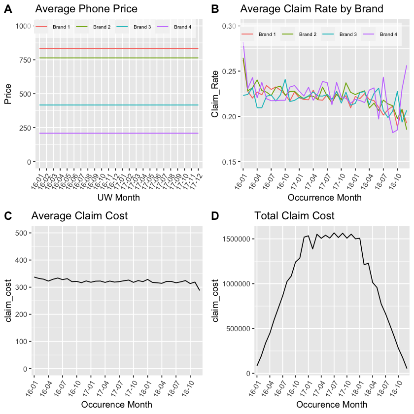
The final set of exhibits are those on slide 44. The only difference of note here is in Chart B, the Claim Rate by phone brand.
Baudry’s exhibits show Brand 1 to have a 5% higher claim frequency than other Brands. From reading the paper I can’t see why we should expect that to be the case. Claim rate varies by phone Model but Model incidence doesn’t vary by Brand. Therefore I can’t see how the Chart B equivalent could be correct given the details in the paper.
I leave the code as is noting the difference but recognising that it will not affect the wider aims of the paper.
Function to create policy and claim data#
The above code can be wrapped into a function which returns a list containing the policy and claim datasets.
By calling the function with a seed you can simulate policy and claim datasets.
tmp <- simulate_central_scenario(1234)

kable(head(tmp$dt_claim), "html") %>%
  kable_styling("striped") %>%
  scroll_box(width = "100%") %>%
  as.character() %>%
  display_html()
| clm_number | pol_number | claim_type | claim_count | claim_sev | date_occur | date_report | date_pay | claim_cost |
|---|---|---|---|---|---|---|---|---|
| 201606080001 | 201601010001 | B | 1 | 0.3337923 | 2016-06-08 | 2016-06-08 | 2016-07-21 | 305 |
| 201609150001 | 201601010014 | B | 1 | 0.3692034 | 2016-09-15 | 2016-09-15 | 2016-10-17 | 309 |
| 201609090001 | 201601010025 | B | 1 | 0.4496012 | 2016-09-09 | 2016-09-09 | 2016-10-07 | 357 |
| 201602190001 | 201601010027 | B | 1 | 0.4019731 | 2016-01-25 | 2016-02-19 | 2016-03-21 | 319 |
| 201605140001 | 201601010043 | B | 1 | 0.2146653 | 2016-05-14 | 2016-05-14 | 2016-06-15 | 196 |
| 201612110001 | 201601010045 | B | 1 | 0.2783313 | 2016-12-11 | 2016-12-11 | 2017-01-06 | 254 |
Download the code and try it yourself#
To finish, if you wish to try out this code in your own local instance of R then we have made this code and the supporting files and folders available in a zip file here.
Download and extract the zip file to a local directory and then open the R project file Baudry_1.rproj in your local R software installation. In the root of the project folder you will see two files;
Notebook_1_SimulateData_v1.Rmd - which is the source code used to recreate this notebook
Notebook_1_SimulateData_v1.R - the equivalent code provided as an R script
Please note that, depending upon your R installation , you may have to install R libraries before you can run the code provided. R will warn you if you have missing dependencies and you can then install them from CRAN.